Project information:
- Introduction
- Methods
- Tasks
- Progress
- References
- Results
Resources:
Sponsor:
Methods
|
We will use a rather simple, yet informative, method
for determining the contributions of the deterministic
and non-deterministic components of the ocean
circulation. This method was proposed by Metzger et al.
[1994], and involves splitting an ensemble of time
series into three constituents:

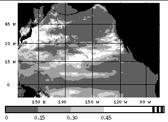
In Figure 2, the relative contributions of the non-deterministic circulation is depicted, based on results from an ensemble of four simulations of the circulation of the Pacific Ocean, using a multi-layer model [Hurlburt and Thompson, 1980; Wallcraft, 1991]. The model, referred as the NRL Layered Ocean Model (NLOM), was driven with the daily surface wind stress product from the ECMWF, and includes effects of realistic bathymetry in the deep ocean. However, the amplitude of the topography above the maximum depth of 6500 m was multiplied by 0.8 to confine it to the lowest layer. The model uses a coastline geometry determined by the 200 m depth contour, which represents the shelf break. |
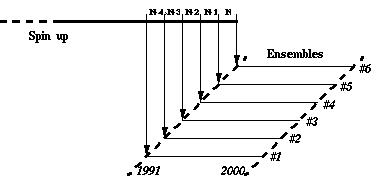
We note that regions that are low in ocean circulation determinism (e.g. the subtropical central Pacific Ocean where Rossby waves are an essential feature, and the region of the Kuroshio Extension which is rich in eddies), show up clearly in Figure 2. We also easily observe that the region of high-latitude ocean eddies in the Gulf of Alaska is relatively low in determinism. With respect to the latter observation, it is emphasized here that the NLOM simulations do not cover the continental shelf, and the shelf slope is only crudely represented in the simulations. Hence, even if the Gulf of Alaska eddies are of a predominantly deterministic nature, the NLOM result will not necessarily reproduce this aspect correctly. Our experiment, which includes a spin-up phase and a suite of six ensemble simulations, is set up completely analogously to the set of NLOM ensemble simulations described above. First, the model is spun up from a state of rest using a monthly wind climatology, on progressively refined horizontal grid meshes. Then, the spin-up phase is extended for a few years, in order to provide a set of initial conditions. Finally, the ensemble simulations are performed with identical wind forcing, with each ensemble receiving its initial values from a different year of the extended spin-up phase. The present strategy for the ensemble simulations is depicted in Figure 3. 
|