Full domain ensemble experiments:
Deterministic vs. nondeterministic sea surface height

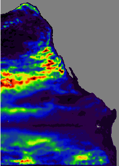
Deterministic vs. non-deterministic sea surface height in the full domain case. Black and purple regions have high degrees of determinism. Green, yellow and red regions have low degrees of determinism. See also the full size figure.

The fraction of non-deterministic variability of the model sea surface height (SSH) is displayed in the figure for the eastern half of the full domain, see the Theory section below. We note that for the main waveguides in this region, which are the equator and the coast, the SSH variability is largely deterministic. In a section from Baja California to California and a section in the GoA, the non-deterministic variability of the SSH along the coast increases relatively rapidly in the off-coast direction. Nevertheless, even these regions exhibits high degrees of determinism in SSH in cells that are adjacent to dry cells. The length scale of the transition from the coastal regions with mostly deterministic SSH to the open ocean regions with relatively low degrees of determinism, is very similar to the internal Rossby radius. This shows that any errors in the model's coastal sea levels (SL) are most likely due to discrepancies in the simulations, such as remote effects which have origins outside the model domain.

Both of these coastal sections are in vicinities of ocean regions which are frequently under the influence of non-linear process such as generation of planetary waves off Baja California and eddies in the GoA. One may suspect that the origins of these instabilities are connected to the coastally trapped signal, and that a loss of a deterministic signal in the oceans' interior should be accompanied by a corresponding loss along the coast. However, the variability of coastal sea levels are almost an order of magnitude larger than those of the sea surface heights in the oceans' interior, so any link between the two in the non-deterministic SSH is overcome by the sustained high amplitude of coastal sea levels.

Theory

In order to assess the degree of determinism in the experiments, an ensemble of four simulations of the FDE was computed for the period 1979-1996. These simulations differed in their initial values only, which were taken from four different years in the model spin-up. Joe Metzger and colleagues at NRL-Stennis have developed a technique to separate the variability of a variable into two components. 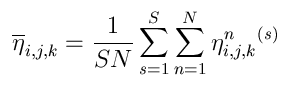(For a complete reference, see the bottom of this page) The deterministic component was interpreted as being due to direct tmospheric forcing, whereas the non-deterministic part is due to onlinear mesoscale flow instabilities. Consider a prognostic variable which varies in space, and define a partitioning of by

(1)

where i,j,k denotes the position in space, n corresponds to time, and s is a realization in the set of ensemble simulations. This separation is described in detail on a separate page. If is a two-dimensional variable, the subscript k should be ignored. Further,

(2)

is the overall mean value for all S realizations as a function of space, and

(3)

is the mean offset among the S realizations from as a function of time. Then, from (1) we see that is the departure in each realization from the instant ensemble mean as a function of space and time, and we have

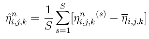
(4)

Using (1) and (3), the variance of the anomaly of , , may be expressed as

(5)

where the overbars on the right hand side are introduced completely analogously to the definition in (2). Keeping in mind that is independent of the variability from one realization to the others, we interpret as the fraction of deterministic variability. The non-deterministic variability fraction is then given as .

Reference
Metzger, E. J., H. E. Hurlburt, G. A. Jacobs, and J. C. Kindle, 1994:
Hindcasting wind-driven anomalies using reduced-gravity global ocean models with 1/2° and 1/4° resolution. NRL Tech. Rep. 9444, 21 pp., Nav. Res. Lab., Stennis Space Center, Miss.