shell scripts:
contour.sh
Syntax
Example 1:
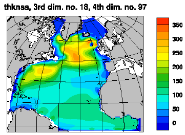
Layer thickness
The figure below was made by issuing the command:
contour.sh 4dmap hycom_031_h.nc thknss 18 97
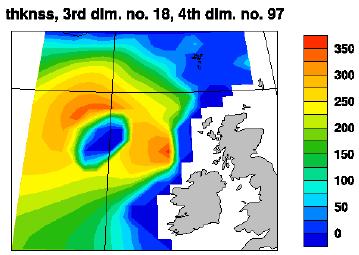
Example 2:
As Example 1, but zooming in
The next figure was made by issuing the same command as in Example 1, after the file userdef.ncl was copied from /home/arnem/lib/ncl-metno/ , with the contents of four lines changed to
x1= 60     ; Leftmost  grid point to depict, for dimension  x  or  lon
x2= 80     ; Rightmost grid point to depict
y1= 85     ; Lowermost grid point to depict, for dimension  y  or  lat
y2= 105    ; Uppermost grid point to depict
in order to zoom in on a sub-domain.
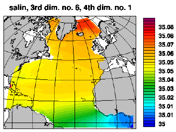
Example 3:
Salinity
Then, a figure was made by issuing the command
contour.sh 4dmap hycom_031_TS.nc salin 6 1
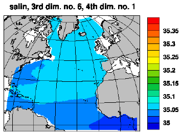
The figure above does not contain a lot of information. This shows that NCL's automatic contouring capability can fall short of the user's requirements. Such a circumstance typically arise when the field to be displayed contains outliers. In this example, salty waters exist south of the tip of Florida. Thus:
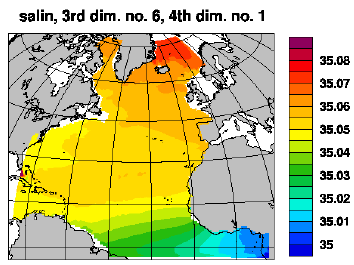
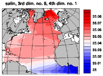
Example 4:
As Example 3, but with more contours and colors
The figure below was made by issuing the same command as in Example 3, after the file userdef.ncl was copied from /home/arnem/lib/ncl-metno/ , with the contents of three lines changed to
v1= 35.00 ; Low  value for isopleths, disregarded when  nv  is 0 or 1
v2= 35.085; High value for isopleths, disregarded when  nv  is 0 or 1
nv= 17    ; No. of isopleths, there will be  nv+1  colors
in order to specify the use of contours and colors.
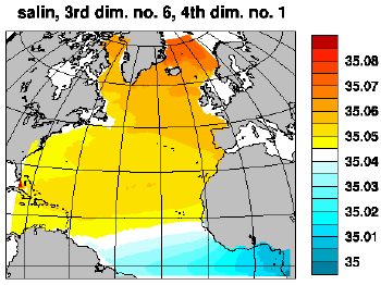
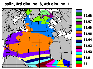
Example 5:
As Example 4, but with even more contours and colors
The figure below was made by issuing the same command as in Example 3, after the file userdef.ncl was copied from /home/arnem/lib/ncl-metno/ , with the contents of three lines changed to
v1= 35.00  ; Low  value for isopleths, disregarded when  nv  is 0 or 1
v2= 35.0875; High value for isopleths, disregarded when  nv  is 0 or 1
nv= 35     ; No. of isopleths, there will be  nv+1  colors
in order to specify the use of contours and colors. Further, an alternative color map was set by editing the contents of two additional lines on the same file, to
;mapname=;"LR BkBlAqGrYeOrReViWh200"; rainbow style, nv <= 17
mapname="HR BkBlAqGrYeOrReViWh200";   rainbow style, nv <= 35
(In ncl, a semicolon [;] is the start of a comment field that extends to the end of the line.)
Note that there is a problem with the labelling of the color bar.
Example 6:
As Example 4, but with different color maps
The figure below was made by issuing the same command as in Example 3, after the file userdef.ncl was copied from /home/arnem/lib/ncl-metno/ , with the contents changed as follows:
Blue/red color map
is specified by editing to
;mapname="LR BkBlAqGrYeOrReViWh200" ; rainbow style,  nv <= 17
mapname="LR BlWhRe"                 ; blue/white/red, nv <= 17
NRL color map
is specified by editing to
;mapname="LR BkBlAqGrYeOrReViWh200" ; rainbow style, nv <= 17
mapname="nrl_sirkes"                ; NRL,           nv <= 17
Gray-scale color map
is specified by editing to
;mapname="LR BkBlAqGrYeOrReViWh200" ; rainbow style, nv <= 17
mapname="gsdtol"                    ; grayscale,     nv <= 17
It may be an idea to change the color of land here...
Tiger stripes color map
is specified by editing to
;mapname="LR BkBlAqGrYeOrReViWh200" ; rainbow style, nv <= 17
mapname="default"                   ; tigerstripes,  nv <= 17
contour.sh: syntax
contour.sh --help

        contour.sh  /  ncl-metno 1.2

>>>
>>>
>>> Syntax:
>>> =======
>>>
>>>  contour.sh <option> <file> <variable> [<d3node> (<d4node>)]
>>> where
>>>    <option>    specifies dimensions and geo- or nongeo-grid
>>>                 implemented:
>>>                  [234]d    - [234]D fields
>>>                  [234]dmap - [234]D fields, dims. are lon & lat
>>>                  [234]dMap - [234]D fields, lon & lat are 2d fields
>>>                  ...[234]d[mM]ap will be displayed on a geogr. map
>>>    <file>      name of the netcdf file
>>>    <variable>  name of requested variable on the netcdf file
>>>                 (case sensitive)
>>>    <d3node>  node no. of third dimension
>>>                if <option> is one of 2d, 2dmap and a fourth
>>>                  argument is present, or if <d3node> is negative,
>>>                  this will be interpreted as a flag that will cause
>>>                  the ncl script to remain (see examples below)
>>>    <d4node>  node no. of fourth dimension
>>>
>>>  Special case:
>>>   If <option> is one of [234]dMap, the name of the 2d longitude and
>>>    latitude variable may be specified on the command line:
>>>   contour.sh <option> <lonname> <latname> <file> <variable> [<d3node> (<d4node>)]
>>>    (Alternatively, if these names are not 'lon' or 'lat', 'userdef.ncl' may
>>>     be edited when option is one of [234]dMap.)
>>>
>>>  The script will produce an eps-file and a png-file.
>>>
>>>
>>> User specifications:
>>> ====================
>>>
>>>  By copying the default spec.s from
>>> /home/arnem/lib/ncl-metno/userdef.ncl
>>>  to the directory where the command 'contour.sh' is given,
>>>  the user may specify
>>>   * title
>>>   * font
>>>   * zooming
>>>   * color map (palette)
>>>   * no. of colors
>>>   * plot size limits
>>>   for geographical maps:
>>>   * names of longitude & latitude variables
>>>   * map projection
>>>   * coastline detail level
>>>  (look up, or copy, this file to edit your own 'userdef' file).
>>>
>>>
>>> Examples:
>>> =========
>>>
>>>  contour.sh 4dmap hydrography.nc temp 1 10
>>>    will produce a depiction on a lon-lat grid w/ a map,
>>>     for the first node in the third dimension (usually
>>>     the top vertical level) and the tenth node in the
>>>     fourth dimension (usually time step no. 10),
>>>     of the variable 'temp' on the file 'hydrography.nc'
>>>  contour.sh 3d surface.nc sst -1
>>>    will produce a depiction on a x-y grid of the first node
>>>     in the third dimension, of the variable 'sst' on the
>>>     file 'surface.nc'; and the ncl-script will be retained
>>>  contour.sh 2dmap topography.nc Depth a
>>>    will produce a depiction on a lon-lat grid w/ a map,
>>>    of the variable 'Depth' on the file 'topography.nc';
>>>     and the ncl-script will be retained
>>>
>>>
>>> Terminating.